Warning: this document is still work in progress. Feel free to send comments but do not consider it final material.

4. Model-based dithering

So far all dithering methods have relied on the assumption that carefully positioned black and white pixels gave the illusion of greyscales, but we have not stated exactly how the human eye reacted. Also, we do not have an automated way to compare the results of two different algorithms: judging that an algorithm is “better” has mostly been a subjective process so far.

In order to figure out what the human eye really sees, we need a human visual system (HVS) model. Countless models exist, and we are only going to focus on simple ones for now.

4.1. Gaussian human visual system model

One of the simplest models is the gaussian HVS model. It states that the human eye acts like a gaussian convolution filter, slightly blurring pixel neighbourhoods and therefore simulating what the eye sees as distance from the image increases. This model, a simplified luminance spatial frequency response formula, can be expressed using the two-dimensional e ^{-(x²+y²)/2σ²} function. The σ parameter sort of introduces the viewing distance into the model.

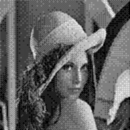
Here are the results of applying a gaussian HVS to an 8×8 Bayer dithered image, simply by convoluting the image with a gaussian blur filter. This process is also known as inverse halftoning. Different values of σ simulate what the eye sees from different distances. On the left σ = 1, on the right σ = 2:

4.2. Direct binary search

We have already seen that standard error diffusion methods do not go back to pixels that have been set. Direct binary search [4] (DBS) is an iterative method that processes the image a fixed number of times, or until the error can no longer be minimised:

• Generate an initial dithered image
• Repeat until no changes can be applied:
  • Compute the global error between the original and the dithered images
  • For each pixel in the dithered image:
    • Compute the effect on the error of toggling the value of the current pixel
    • Compute the effect on the error of swapping the current pixel with one of its immediate neighbours
    • If the error can be reduced, perform the corresponding action

The efficiency and quality of DBS depend on many implementation details, starting with the HVS model it uses to compute the error. Also, the initial image used as iteration zero will give poor results if pattern artifacts are already present. The order in which pixels are processed is important, too. Unfortunately, despite its very high-quality results, DBS is usually a very slow algorithm.

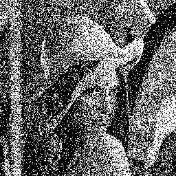
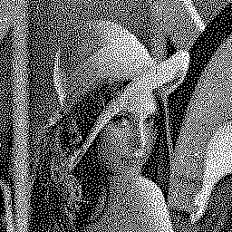
Below is an example of the algorithm results. The HVS uses a 11×11 convolution kernel of the e ^{-sqrt(x²+y²)} function. The initial image is randomly thresholded, and pixels are processed in raster order. Iterations 1, 2 and 5 are shown:

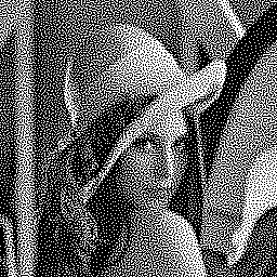
Other HVS models can be used, giving very high quality results. Below are the results of DBS with the following HVS functions:

• e ^-(x²+y²)/2
• e ^{-(x²+y²)/4.5}
• e ^-(x²+y²)/8
• 2e ^{-(x²+y²)/1.5} + e ^-(x²+y²)/8

The iteration shown is number 5. More iterations would have improved the results even slightly more, but that would have been at the expense of performance:

4.3 Comparing dithering algorithms

Using an HVS model, it is possible to classify previously seen algorithms simply by applying the model to both the source and the destination images, and computing their per-pixel mean squared error. This gives a better estimation of the dithering algorithm’s quality than simply computing a local, pixel-bound error.

The following table shows that different HVS models give very different error values depending on the value of σ. Also, in the case of the DBS algorithm, a carefully crafted HVS function such as the last one, which combines two different HVS models, gives low error values at every σ, which means the dithered image is close to the original image at all corresponding viewing distances: